Matthias Broecheler
CEO of DataSQRL
View all authors

AI in Data Engineering: Building Reliable Data Systems at Scale

· 13 min read
Matthias Broecheler
CEO of DataSQRL

AI is transforming data engineering. Coding agents can now generate SQL transformations, configure connectors, and define API schemas in minutes rather than days. But here's the catch: a query that works perfectly on test data may fail catastrophically when confronted with late-arriving events, schema evolution, or terabyte-scale volumes.

How do we ensure that AI-generated data systems meet the rigorous non-functional requirements that production data platforms demand? This article presents our framework for integrating AI coding agents into data engineering workflows while maintaining data quality, reliability, governance, and trust.

The Scaling Challenge

Organizations are targeting 3-5x productivity improvements through AI-assisted development. The velocity is real, but it creates an unsustainable burden on traditional data engineering practices:

  • Manual code review can't scale when agents generate dozens of pipeline changes daily
  • Ad-hoc data quality checks miss subtle issues that only manifest at scale or over time
  • Tribal knowledge about production constraints doesn't transfer to AI agents
  • Integration testing becomes a bottleneck when deployment velocity outpaces validation capacity
  • Operations and troubleshooting overwhelm teams when they have to manage dozens of pipelines in production

The fundamental problem is coding agents optimize for functional correctness (e.g. does the query return the right results?) while production data systems require a much broader set of guarantees.

Without systematic guardrails, AI-generated data pipelines work in demos but fail in production and overwhelm the data engineering teams that have to fill the gaps.

A Data Quality Governance Framework

Successfully integrating AI into data engineering requires a governance framework that addresses three dimensions: transparency, validation, and operations.

Transparency: Exposing Data Lineage and Reasoning

AI agents need to operate within systems that expose their reasoning and the data flows they create. This serves two purposes: enabling human oversight and providing feedback for iterative refinement.

What does transparency look like for data engineering?

  • Clear Transformations: Well-defined data transformations that make it obvious what was transformed and why
  • Data lineage tracking: Trace every output field back through transformations to source systems
  • Computational DAGs: Visualize how data flows from ingestion through processing to serving
  • Schema inference: Make explicit the types, keys, and timestamps the agent has assumed
  • Execution plans: Show which engines execute which computations

When an agent proposes a data pipeline, we should see not just the SQL code but the complete picture: where data originates, how it transforms, what guarantees apply at each stage, and how it ultimately reaches consumers.

=== SpendingTransactions
ID: default_catalog.default_database.SpendingTransactions
Type: stream
Stage: flink
Inputs: Transactions, Accounts, AccountHolders

Annotations:
- temporal-join: uses event-time semantics
- stream-root: Transactions

Primary Key: transactionId, tx_time
Timestamp : tx_time

Schema:
- transactionId: BIGINT NOT NULL
- amount: DECIMAL(10,2) NOT NULL
- tx_time: TIMESTAMP_LTZ(3) *ROWTIME* NOT NULL
- creditor_name: VARCHAR NOT NULL

This representation combines inferences from the logical layer (primary keys, timestamps) with physical mappings (execution stage, inputs) to give us complete visibility into agent-generated pipelines.

Validation: Real-Time Quality Assessment

Every agent action must pass through validation layers that assess correctness before execution. Here's what makes data pipelines different from application code: bugs often produce silently wrong results: queries that execute successfully but return incorrect data.

Effective validation operates at multiple levels:

Logical Validation

  • Syntax and schema verification
  • Data type inference and consistency checking
  • Primary key and timestamp propagation validation
  • Table type verification (stream vs. state semantics)

Physical Validation

  • Engine capability matching (can Postgres execute this temporal join?)
  • Data type mapping consistency across engines
  • Connector configuration verification
  • Topological constraint satisfaction (data must reach database before API can serve it)

Semantic Validation

  • Business rule assertions
  • Data quality constraints (nullability, referential integrity, value ranges)
  • SLA verification (latency bounds, freshness guarantees)

The validation system needs to provide actionable feedback when checks fail. Rather than cryptic error messages, agents need comprehensive context and suggested fixes:

ERROR: Temporal join requires timestamp column on probe side

Table 'Transactions' is used in a temporal join with 'Accounts'
but lacks a rowtime attribute.

Suggestion: Add a timestamp column with WATERMARK definition:
tx_time TIMESTAMP_LTZ(3),
WATERMARK FOR tx_time AS tx_time - INTERVAL '5' SECOND

Operations: Continuous Monitoring and Autonomous Troubleshooting

Building pipelines is only half the challenge. When you're managing dozens of AI-generated data pipelines in production, operations becomes the bottleneck. Traditional monitoring approaches (dashboards, manual alerts, runbooks) can't scale when pipeline count grows faster than team headcount.

The framework needs to support autonomous operations:

Continuous Monitoring

  • Real-time data quality assertions that validate business rules on every record
  • SLA tracking that measures end-to-end latency from source event to API availability
  • Schema drift detection that catches upstream changes before they break downstream consumers
  • Resource utilization monitoring that identifies capacity issues before they cause failures

Autonomous Troubleshooting

  • Automatic correlation of symptoms to root causes using lineage information
  • Self-healing for common failure modes (connector reconnection, checkpoint recovery, partition rebalancing)
  • Intelligent alerting that groups related issues and suppresses noise
  • Runbook automation that executes standard remediation steps without human intervention

Observability Integration

  • Structured logging that links every record to its source transformation
  • Distributed tracing across the complete pipeline (Kafka → Flink → Postgres → API)
  • Metrics export to existing observability platforms (Prometheus, Datadog, CloudWatch)

The goal is a team of three data engineers being able to operate dozens pipelines in production. That's only possible when the harness handles routine operations autonomously and escalates only the issues that genuinely require human judgment.

Capturing Data Engineering Expertise

The effectiveness of AI in data engineering depends on systematically capturing and encoding human expertise. This falls into three categories: domain knowledge, operational patterns, and failure modes.

Domain Knowledge Encoding

Data engineers carry implicit knowledge about their data domains: which fields contain PII, how upstream systems behave during maintenance windows, what query patterns consumers actually use. This knowledge needs to be made explicit for agents to leverage.

What works:

  • Schema annotations: Capture business semantics beyond technical types
  • Data contracts: Formalize expectations between producers and consumers
  • Quality rules: Encode domain-specific validity constraints
  • Access patterns: Document how data gets queried in practice
-- Domain knowledge encoded in table definition
/** Customer spending transactions enriched with merchant details.
PII: contains customer_id (indirect identifier)
Freshness SLA: < 5 minutes from source event
Primary consumer: Fraud detection system (latency-sensitive)
*/
SpendingTransactions := SELECT ...

Operational Pattern Libraries

Production data pipelines exhibit recurring patterns: CDC deduplication, temporal enrichment joins, windowed aggregations, slowly changing dimensions. We encode them as reusable patterns to reduce the occurrence of subtle bugs when agents try to recreate them.

-- Pattern: CDC deduplication to current state
Accounts := DISTINCT AccountsCDC ON account_id ORDER BY update_time DESC;

-- Pattern: Temporal enrichment join
EnrichedTransactions := SELECT t.*, a.account_type
FROM Transactions t
JOIN Accounts FOR SYSTEM_TIME AS OF t.tx_time a
ON t.account_id = a.account_id;

-- Pattern: Tumbling window aggregation
HourlyMetrics := SELECT
window_start, COUNT(*) as event_count
FROM TABLE(TUMBLE(TABLE Events, DESCRIPTOR(event_time), INTERVAL '1' HOUR))
GROUP BY window_start;

These patterns encode not just the SQL syntax but the semantic intent and operational characteristics. When an agent needs CDC deduplication, it applies the established pattern rather than improvising a potentially incorrect solution.

Failure Mode Documentation

Every production incident represents encoded knowledge about what can go wrong. Systematically capturing failure modes and their resolutions creates a corpus that agents can learn from:

  • Symptoms: How the failure manifested (data delays, incorrect aggregates, schema mismatches)
  • Root cause: The underlying issue (late data handling, join key mismatch, type coercion)
  • Resolution: How we fixed it
  • Prevention: What validation or pattern would have caught this earlier

Over time, this corpus enables agents to anticipate failure modes and proactively avoid them.

The Data Engineering Harness

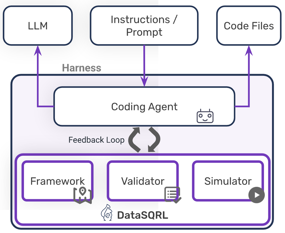
Implementing governance, validation, and expertise capture requires purpose-built infrastructure. We call this a data engineering harness: a system that provides the guardrails and feedback loops coding agents need to produce production-grade data systems.

Data engineering harness architecture

The harness has three integrated components:

Conceptual Framework

The framework provides a precise vocabulary for reasoning about data transformations:

Logical Layer: Expresses what transformations are needed using SQL extended with stream processing semantics. The declarative nature enables deep introspection. We can analyze query structure, infer schemas, and validate semantics.

Physical Layer: Represents how data gets processed through engine assignment and configuration. A cost-based optimizer maps logical operations to physical engines (Flink, Kafka, Postgres, Iceberg) while respecting capability constraints.

Why does this separation matter? Agents should reason about business logic (logical layer) while the harness handles infrastructure complexity (physical layer). This division produces higher quality results by keeping agent context focused on the problem domain.

Comprehensive Validation

Validation operates continuously throughout the development lifecycle:

  • Compile-time: Schema consistency, type safety, semantic correctness
  • Plan-time: Physical feasibility, capability matching, optimization validity
  • Test-time: Functional correctness against known inputs and expected outputs
  • Deploy-time: Configuration validity, resource availability, dependency satisfaction
  • Run-time: Data quality assertions, SLA monitoring, anomaly detection

Each validation stage produces structured feedback that agents consume for iterative refinement. The harness transforms validation failures into actionable guidance.

Real-World Feedback

Static validation catches many issues but can't substitute for execution feedback. The harness provides two mechanisms for real-world validation:

Simulation: Execute pipelines locally with timestamp-accurate event replay. The simulator runs the complete stack (Flink, Kafka, Postgres) in Docker, enabling agents to test against realistic data volumes and timing scenarios. Crucially, simulation is deterministic: the same inputs always produce the same outputs, enabling reliable regression testing.

Production Telemetry: Monitor deployed pipelines and correlate observations back to source code. When latency increases or data quality degrades, the harness links metrics to specific transformations, enabling autonomous troubleshooting.

Feedback loops from harness components back to coding agent

Implementation: The DataSQRL Approach

DataSQRL implements this harness architecture as an open-source framework. Here's how the abstract governance principles translate to concrete tooling.

SQL as the Logical Layer

DataSQRL uses SQRL as the logical representation, which is SQL extended with stream processing from Flink SQL and interface definitions. Why SQL?

  • LLM familiarity: Most models are extensively trained on SQL
  • Human readability: Engineers can verify agent output without learning new syntax
  • Mathematical foundation: Relational algebra enables rigorous validation
  • Declarative introspection: We can analyze and transform queries programmatically
-- Agent-generated pipeline in SQRL
IMPORT banking_data.*;

-- Deduplicate CDC stream to current state
Accounts := DISTINCT AccountsCDC ON account_id ORDER BY update_time DESC;

-- Enrich transactions with temporal join
SpendingTransactions := SELECT
t.*,
h.name AS creditor_name
FROM Transactions t
JOIN Accounts FOR SYSTEM_TIME AS OF t.tx_time a
ON t.credit_account_id = a.account_id
JOIN AccountHolders FOR SYSTEM_TIME AS OF t.tx_time h
ON a.holder_id = h.holder_id;

-- Define API endpoint
SpendingByAccount(account_id STRING NOT NULL) :=
SELECT * FROM SpendingTransactions
WHERE debit_account_id = :account_id
ORDER BY tx_time DESC;

Deterministic Transpilation

The mapping from logical to physical layer happens through deterministic transpilation, not agent generation. This eliminates an entire class of subtle bugs:

  • Schema mismatches between engines
  • Incorrect data type coercions
  • Missing index structures
  • Inconsistent serialization formats

The transpiler generates deployment artifacts (Flink plans, Kafka topics, Postgres schemas, GraphQL models) that are guaranteed consistent with the logical definition. Agents focus on business logic while the harness handles infrastructure integration.

Complete framework showing transpilation from SQL to multiple engines

Neuro-Symbolic Optimization

Certain data engineering tasks are better handled by dedicated optimizers than LLM reasoning. DataSQRL implements a neuro-symbolic approach: agents handle high-level design while specialized solvers handle constraint satisfaction.

  • Query Optimization: Apache Calcite's Volcano optimizer rewrites queries for performance
  • Physical Planning: Cost-based optimizer assigns operations to engines while respecting topological constraints
  • Index Selection: Lattice-based optimizer selects index structures that support query access patterns

Agents can provide hints to guide optimization (e.g. forcing specific engine assignments or partition keys) but the optimizer ensures constraint satisfaction. This leverages LLM strengths (reasoning under uncertainty, creative problem-solving) while delegating deterministic optimization to purpose-built systems.

Continuous Evaluation

The harness supports continuous evaluation through automated testing infrastructure:

/*+test */
TransactionEnrichmentTest :=
SELECT creditor_name, COUNT(*) as tx_count
FROM SpendingTransactions
GROUP BY creditor_name
ORDER BY creditor_name;

Test definitions execute against known inputs with expected outputs captured as snapshots. The simulator replays events with precise timestamps, enabling tests for complex scenarios:

  • Late-arriving events and watermark handling
  • Out-of-order data processing
  • Race conditions in temporal joins
  • Schema evolution compatibility

Tests provide immediate feedback to agents and spot regressions in CI/CD infrastructure.

Organizational Implications

Successfully integrating AI into data engineering requires organizational adaptation beyond tooling. What shifts as AI assumes greater responsibility for pipeline development?

From Implementation to Oversight

As agents handle routine implementation, data engineers shift focus toward:

  • Architecture review: Evaluating agent-proposed designs against organizational patterns
  • Pipeline auditing: Reviewing agent-generated pipelines for correctness, efficiency, and compliance
  • Domain encoding: Capturing business knowledge in schemas, contracts, and quality rules
  • Failure analysis: Investigating production issues and encoding learnings
  • Governance evolution: Refining validation rules and operational criteria

This shift parallels the evolution in other engineering disciplines where automation handles routine tasks while humans focus on judgment-intensive decisions.

From Manual Testing to Continuous Validation

Traditional data pipeline testing, manual verification against sample datasets, can't scale with AI-accelerated development. Organizations need to invest in:

  • Comprehensive test suites that encode expected behavior across edge cases
  • Automated regression detection that flags behavioral changes between versions
  • Production monitoring that validates data quality continuously
  • Anomaly detection that identifies novel failure modes

The testing burden shifts from per-deployment verification to continuous infrastructure maintenance.

From Tribal Knowledge to Encoded Expertise

AI agents can't access knowledge that exists only in engineers' heads. Organizations need to systematically externalize:

  • Data domain semantics and business rules
  • Operational patterns and anti-patterns
  • Historical failure modes and resolutions
  • Consumer requirements and SLAs

This documentation effort has value beyond AI enablement: it improves onboarding, reduces key-person dependencies, and creates institutional memory that persists through team changes.

The Path Forward

AI-assisted data engineering is here. Organizations that successfully integrate AI into their data platforms will achieve significant productivity gains while maintaining the reliability that production systems demand.

AI integration requires infrastructure, not just tools. Coding agents operating without guardrails produce pipelines that work in demos but fail in production. Agents operating within a purpose-built harness with comprehensive validation, real-world feedback, and encoded expertise produce pipelines that meet production requirements.

The data engineering harness represents this infrastructure: a system that provides the governance, validation, and feedback loops necessary for AI-assisted data platform automation.

DataSQRL implements this harness as an open-source framework. You can customize it to encode your domain knowledge, integrate your validation rules, and build an automated data platform tailored to your requirements.

The question is no longer whether AI will transform data engineering, but how we adapt our practices, tooling, and teams to harness its potential while maintaining the trust that data consumers depend on.

Getting Started

To explore AI-assisted data engineering with DataSQRL:

  1. Build a project from scratch to understand harness components
  2. Explore example projects demonstrating common patterns
  3. Read about the harness architecture for detailed technical background
  4. Contribute to the open-source project to shape the future of AI-assisted data engineering

Agentic Data Engineering Harness

· 19 min read
Matthias Broecheler
CEO of DataSQRL

DataSQRL is an open-source data engineering harness that provides guardrails and feedback for AI coding agents to develop and operate data pipelines, data products, and data APIs autonomously. You can customize DataSQRL as the foundation of your agentic data platform. Our goal is to develop DataSQRL into a comprehensive data engineering harness for data platform automation.

DataSQRL harness architecture showing coding agent with framework, validator, and simulator feedback loops >

Why a Data Engineering Harness?

Coding agents are transforming software development. Tools like Claude Code, Copilot, and Codex can generate application code, write tests, and even refactor entire codebases. But data engineering presents unique challenges that general-purpose coding agents struggle to address.

The difference lies in non-functional requirements. When you build a data pipeline, functional correctness (does the query return the right results?) is just the starting point. Production data systems must also deliver:

  • Data Quality: Consistent, accurate data with proper handling of late-arriving events, duplicates, and schema evolution
  • Scalability: Performance that holds up as data volumes grow from gigabytes to terabytes
  • Governance: Lineage tracking, access controls, and audit trails for regulatory compliance
  • Reliability: Exactly-once semantics, failure recovery, and graceful degradation under load
  • Cost Efficiency: Optimal resource utilization across compute, storage, and network

A coding agent can generate a SQL query that produces correct results on a test dataset. But will that query perform at scale? Does it handle late data correctly? Will it maintain data quality guarantees when upstream schemas change? These are the questions that justify data engineering as its own discipline and that general-purpose coding agents are not equipped to answer consistently.

A data engineering harness provides the guardrails, feedback loops, and domain-specific constraints that coding agents need to produce production-grade data systems. Without a harness, you get code that works in demos but fails in production. With a harness, you get data pipelines that embody decades of hard-won data engineering and domain-specific knowledge.

DataSQRL is that harness. It encodes the conceptual framework of data systems, validates implementations against data engineering best practices, and provides real-world feedback through simulation and production telemetry. The goal is to constrain coding agents into building data systems you'd actually trust to run in production.

The DataSQRL Harness

Feedback loops from framework, compiler, testing, validators, and runtime back to the coding agent

For the purposes of automating data platforms, a comprehensive harness captures data schemas, data processing, and data serving to consumers. Specifically, we are building a harness for non-transactional data processing and serving.

The harness provides the frame of reference for implementing safe, reliable data processing systems. It captures the knowledge from Database Systems: The Complete Book combined with 25 years of data engineering experience.

DataSQRL breaks the harness into logical and physical layers.

Logical Layer

The logical layer expresses what data transformations are needed to produce the desired results.

An obvious choice for the logical layer is Codd's relational model and its most popular implementation SQL.

The relational model is widely adopted, proven, and provides a solid mathematical foundation. Most LLMs are trained on lots of SQL code and related documentation. And it is easy for humans to read. Modern versions of SQL (e.g., the SQL:2023 standard) support semi-structured data (JSON), polymorphic table functions, and complex pattern matching to address the messy reality of data platforms.

While the relational model and SQL are a good starting point, we need two additions to achieve the expressibility that modern data platforms require.

1. Dataflow

The relational model uses set semantics. That is inconvenient for representing data flows which are important for data pipelines.

Jennifer Widom's Continuous Query Language extends the relational model with data streams and relational operators for moving between streams and sets.

Flink SQL, based on Apache Calcite, is the most widely adopted implementation of this extended relational model. That's why we use Flink SQL as the basis of the logical layer in DataSQRL.

Using a declarative language for the harness has a number of advantages from concise representation to deep introspection, but a practical shortcoming is the fact that some data transformations are easier to express imperatively. Flink SQL overcomes this by supporting user defined functions and custom table operators in programming languages like Java. This gives us a logical layer grounded in relational algebra with flexible extensibility to express complex data transformations imperatively.

DataSQRL builds on Flink SQL and adds 1) concise syntax for common transformations, 2) dbt-style templating, and 3) modular file management and importing. These features help with context management for LLMs by reducing the size of the active context that needs to be maintained during implementation and refinement.

-- Ingest data from connected systems
IMPORT banking_data.AccountHoldersCDC; -- CDC stream from masterdata
IMPORT banking_data.AccountsCDC; -- CDC stream from database
IMPORT banking_data.Transactions; -- Kafka topic for transactions

-- Convert the CDC stream of updates to the most recent version
Accounts := DISTINCT AccountsCDC ON account_id ORDER BY update_time DESC;
AccountHolders := DISTINCT AccountHoldersCDC ON holder_id ORDER BY update_time DESC;

-- Enrich debit transactions with creditor information using time-consistent join
SpendingTransactions :=
SELECT
t.*,
h.name AS creditor_name,
h.type AS creditor_type
FROM Transactions t
JOIN Accounts FOR SYSTEM_TIME AS OF t.tx_time a
ON t.credit_account_id = a.account_id
JOIN AccountHolders FOR SYSTEM_TIME AS OF t.tx_time h
ON a.holder_id = h.holder_id;

We call this SQL dialect SQRL. You can read the documentation for a complete reference of the SQRL language.

2. Serving

In addition to data processing, a critical function of data platforms is serving data to consumers as data streams, datasets, or data APIs. Data APIs, in particular, are becoming more important with the rise of operational analytics and MCP (Model Context Protocol) for making data accessible to AI agents.

To support data serving, DataSQRL adds support for endpoint definitions via table functions and explicit relationships.

Table functions are part of the SQL:2016 standard and return entire tables as result sets computed dynamically based on provided parameters. In DataSQRL, table functions can be defined as API entry points.

/** Retrieve spending transactions within the given time-range.
from_time (inclusive) and to_time (exclusive) must be RFC-3339 compliant date time.
*/
SpendingTransactionsByTime(
account_id STRING NOT NULL METADATA FROM 'auth.accountId',
from_time TIMESTAMP NOT NULL,
to_time TIMESTAMP NOT NULL
) :=
SELECT * FROM SpendingTransactions
WHERE debit_account_id = :account_id
AND :from_time <= tx_time
AND :to_time > tx_time
ORDER BY tx_time DESC;

Furthermore, DataSQRL allows for explicit relationship definitions between tables which are important for API-based data access where results need to include related entities like most recent orders or recommendations for movie category. The relational model does not support traversing through an entity-relationship model, which is usually handled by an object-relational mapping layer when exposing an API. To avoid that extra complexity and impedance mismatch in our logical layer, DataSQRL provides first-class support for relationships.

-- Create a relationship between holder and accounts filtered by status
AccountHolders.accounts(status STRING) :=
SELECT * FROM Accounts a
WHERE a.holder_id = this.holder_id
AND a.status = :status
ORDER BY a.account_type ASC;

With the addition of access functions and relationships, the logical layer maps directly to the entity-relationship model of GraphQL which DataSQRL uses as the logical representation for API-based data retrieval. This gives DataSQRL a highly expressive interface with a simple extension of the logical layer which retains conceptual simplicity of the harness.

The interface documentation provides more details on the serving layer of DataSQRL.

Physical Layer

The physical layer represents how the data gets processed and served. It's a translation of the logical layer into executable code that runs on actual data systems.

Complete DataSQRL framework showing data flow from sources through processing, storage, and serving layers

Pipeline Architecture

With hundreds of database systems and many more data infrastructure choices, it is a daunting challenge to construct a simple and coherent physical layer that is flexible enough to cover the diverse needs of data platforms.

After analyzing a wide range of data platforms, we identified that the vast majority of implementations combine multiple data systems from these categories:

  • Database: for storing and querying data, e.g., PostgreSQL, MySQL, SQLServer, Apache Cassandra, Clickhouse, etc.
    • Table Formats and Query Engines: For analytic data, separating compute from storage can save money and support multiple consumers. DataSQRL conceptualizes this as a "disintegrated database" with table formats for storage (e.g., Apache Iceberg, DeltaLake, Apache Hudi) and query engines for access (e.g., Apache Spark, Apache Flink, Snowflake).
  • Data Processor: for batch or realtime transformation of data, e.g., Apache Spark, Apache Flink, etc.
  • Log/Queue: for reliably capturing data and moving it between data systems, e.g., Apache Kafka, RedPanda, Kinesis, etc.
  • Server: for capturing and exposing data through an API
    • Cache: sits between server and database to speed up frequent queries over less-frequently changing data.

We call each data system an engine and the above categories engine types. When looking at data platform implementations at the level of engine types, we see about 15 patterns emerge (the 10 most popular are documented here) that arrange those engines in a directed-acyclic graph (DAG) of data processing.

Hence, we use a computational DAG that models the flow of data from source to interface as the basis of our physical layer. Each node in the DAG represents a logical computation mapped to be executed by an engine. Thus, the physical layer provides an integrated view of the entire data flow.

Transpiler

While the physical layer gives the AI control over what engine executes which computation, the actual mapping of logical to physical plan is done by a deterministic transpiler built in Apache Calcite. This avoids subtle bugs in data mapping and execution. The results of the transpilation are deployment assets which are executed by each engine. For example, the transpiler generates the database schema and queries for Postgres.

In the transpiler component, we make the following simplifying assumptions:

  • The database engines support a version of SQL (e.g., PostgreSQL, T-SQL) or a subset thereof (e.g., Cassandra Query Language)
  • The data processor supports a SQL-based dialect (e.g., Spark SQL, Flink SQL)
  • The log engine is Apache Kafka compatible (e.g., RedPanda, Azure EventHub)
  • The server has a GraphQL execution engine.

This modular architecture allows new engines to be added by conforming to the engine type interface and implementing the transpiler rules in Calcite where needed. At the same time, it abstracts much of the physical plan mapping complexity from the AI, which produces higher quality results and preserves context for higher-level reasoning.

Configuration

DataSQRL uses a package.json file to configure the engines used to execute a data pipeline. The configuration file defines the overall pipeline topology, the individual engine configurations, and the compiler configuration. One file controls how the physical layer is derived and executed, making it simple for the AI to experiment with and fine-tune the physical layer.

Interface

For the data serving interface, we use GraphQL schema as the physical representation which bidirectionally maps to the access functions, table schema, and relationships defined in the logical plan by naming convention. GraphQL fields are mapped to SQL or Kafka queries based on their respective definitions in SQRL. This allows the AI to fine-tune the API within the GraphQL schema.

Furthermore, REST and MCP APIs can be explicitly or implicitly defined through GraphQL operations. Implicit definition traverses the GraphQL schema from root query and mutation fields. Explicitly defined operations are provided as separate GraphQL files.

Using GraphQL as the physical representation for the API combines simplicity with flexibility while benefiting from the prevalence of GraphQL in LLM training data.

Validator

The harness gives AI coding agents a frame of reference to reason about data pipeline and data product implementations. DataSQRL provides validation to support that reasoning and give users tools to ensure the correctness and quality of the generated pipelines and APIs.

Verification & Introspection

Verification and introspection complement the harness by reinforcing the concepts, rules, and dependencies. DataSQRL provides validation at 3 levels: the logical layer, physical layer, and deployment assets (the code that gets executed by the engines).

Logical

At the logical level, the DataSQRL compiler verifies syntax, schemas, and data flow semantics. This ensures that the data pipeline is logically coherent and that data integration points (e.g., between the SQL definitions and GraphQL schema) are consistent.

One of the benefits of using relational algebra as the basis for our harness is the ability to run rules and deep traversals over the operators in the relational algebra tree. The DataSQRL compiler uses Apache Calcite's rule and RelNode traversal framework to validate timestamp propagation, infer primary keys and data types, validate table types, and more. This validation component can be extended with custom rules to validate domain-specific semantics and constraints.

The validation component was designed to provide comprehensive context and suggested fixes for validation errors. In our testing, this produces significantly better results compared to the AI coding agent having to look up and reason about encountered errors.

Physical

On compilation, DataSQRL produces the computational data flow DAG that represents the physical layer. DataSQRL generates a visual representation as shown above for human validation as well as a concise textual representation that is consumed by coding agents as feedback on their proposed solutions and to reinforce the conceptual data flow of the harness.

=== CustomerTransaction
ID: default_catalog.default_database.CustomerTransaction
Type: stream
Stage: flink
Inputs: default_catalog.default_database._CardAssignment, default_catalog.default_database._Merchant, default_catalog.sources.Transaction
Annotations:
- stream-root: Transaction
Primary Key: transactionId, time
Timestamp : time
Schema:
- transactionId: BIGINT NOT NULL
- cardNo: VARCHAR(2147483647) CHARACTER SET "UTF-16LE" NOT NULL
- time: TIMESTAMP_LTZ(3) *ROWTIME* NOT NULL
- amount: DOUBLE NOT NULL
- merchantName: VARCHAR(2147483647) CHARACTER SET "UTF-16LE" NOT NULL
- category: VARCHAR(2147483647) CHARACTER SET "UTF-16LE" NOT NULL
- customerId: BIGINT NOT NULL

This representation of the physical layer combines the inferences from the logical layer with the mapping to execution engines to provide a source-to-interface definition of the data flow.

Validation at the physical level ensures that data type mappings are consistent and that the engine assignments are valid, i.e., that an assigned engine has the capabilities to execute a particular operator. DataSQRL uses a capabilities component that extracts all requirements from an operator (e.g., temporal join, or a particular function execution) and validates that the engine supports the corresponding capabilities.

Deployment Assets

The executable deployment assets are transpiled from the physical layer. Since the transpilation is deterministic, this yields better results than letting the coding agent generate them, and it keeps the harness concise. However, we generate all deployment assets in a text representation that the coding agent can easily consume as another source of feedback. This is particularly useful during troubleshooting where the deployment assets are the ultimate source of truth of what is being executed and allow the agent to reason "backwards" to the logical layer and how to fix it.

Specifically, we generate:

  • Database: The database schema, index structures, and (parameterized) SQL queries for all views and API entrypoints.
  • Data Processor: The optimized physical plan and compiled execution plan.
  • Log: The topic definitions and filter predicates.
  • Server: The mapping from GraphQL fields to database or Kafka queries as well as operation definitions. Also, the GraphQL schema if it is not provided.

Optimization

While LLMs' reasoning ability under uncertainty is outstanding, we have found LLMs to perform worse and less consistently on deterministic optimization and constraint satisfaction problems. This finding is supported by a rich body of research in neuro-symbolic AI which researches the integration of neural networks (like LLMs) with symbolic computation (e.g., solvers, planners) and has documented how neural networks alone fall short for such tasks.

DataSQRL follows the neuro-symbolic approach and provides 3 types of planners for deterministic sub-tasks in the implementation and maintenance of data pipelines:

Query Optimization

Query rewriting and optimization is a well-established technique for producing high-performing physical plans from relational algebra. DataSQRL relies on Apache Calcite's Volcano optimizer and HEP rule engine for this purpose.

Physical Planning

The physical plan DAG is subject to a number of constraints forced by the real-world constraints of physical data movement. For example, when the API needs to serve data on request, that data must first be available in the database. It cannot be served directly from a data processor. These topological constraints combined with the capabilities of individual engines render many AI-proposed solutions invalid.

Hence, we implement a physical planner that uses a cost model with a greedy heuristic to assign logical operators to engines in a way that is consistent. The AI can provide hints to force the assignment of certain operators to specific engines which are added as constraints to the optimizer. This gives the AI control over allocations but shifts the burden of constraint satisfaction to a dedicated solver.

Index Selection

Efficiently querying data in the database or table format requires index structures (or partition + sort keys) that support the access paths to the data. Otherwise, we execute inefficient table scans.

Index structure selection is another optimization problem that is better handled by a dedicated optimizer. We use an adaptation of Ullman et al's lattice framework for data cube selection since data cube selection and index selection are related problems with different optimization functions.

Real World Feedback

A harness with complementary verification and introspection provides the foundation of a concise model for data pipelines with feedback on proposed solutions. However, that feedback is limited to the plan and does not account for the complexities of actual execution. Real-world feedback is critical for iterative refinement of production-grade implementations and troubleshooting issues that arise in operation.

DataSQRL provides two sources of real-world feedback: a simulator that's used at implementation time and telemetry collection from production deployments that captures the operational status of the pipeline.

Simulator

The DataSQRL simulator executes the configured engines with the generated deployment assets within a Docker environment. The simulator can replay events and records at their original timestamp, allowing for deterministic reproducibility of real-world scenarios. This is important for creating realistic test cases as well as reproducing production issues for troubleshooting and regression testing.

By capturing and faithfully replaying records at their original timestamp, the simulator ensures time-consistent semantics of data flows and makes it simple to construct complex test cases for scenarios like race conditions.

Simulation is important in agentic coding workflows because it allows the agent to execute and refine the implementation in a feedback loop that is executed locally and can simulate scenarios that only occur rarely in production.

Read more about invoking the simulator and writing reproducible test cases.

Operations and Telemetry

The most important source of real-world feedback is observing the deployed data pipeline in a production environment (or a closely approximated pre-prod environment). Observability is critical for assessing the health of the pipeline and troubleshooting any issues that may occur.

Logs and telemetry collection is a well-established practice for DevOps. What DataSQRL adds is the ability to link observed data back to the physical computation DAG so the agent can accurately reason about cause and effect. For data pipelines that execute across multiple engines, many complex errors arise at system boundaries and require reasoning across multiple systems. For example, an issue in the data processing layer may cause excessive writes to the database, degrading overall performance. To automate such troubleshooting, we need to correlate observations back to the physical data flow and logical layer.

DataSQRL currently assumes production operation in Kubernetes or Docker and provides hooks for extracting logs and telemetry data. That data is correlated back to the SQL code and configuration defining the pipeline via the deployment assets, allowing coding agents to reason about effective solutions for troubleshooting production issues autonomously.

Summary

Data engineering is entering a new era of automation. Coding agents can now write SQL, configure pipelines, and deploy data systems. But without proper guardrails, they produce solutions that fail under the weight of production requirements.

DataSQRL is the data engineering harness that ensures AI coding agents produce high-quality pipelines. DataSQRl encodes decades of data engineering knowledge into a structured framework that coding agents can leverage to build production-grade data systems.

The harness provides three critical capabilities:

  1. A Conceptual Framework grounded in relational algebra and stream processing that gives agents a precise vocabulary for reasoning about data transformations, with logical and physical layers that separate what from how.

  2. Comprehensive Validation at every level ensures that agent-generated code meets data engineering standards before it reaches production: from syntax and schema validation through physical plan verification to deployment asset generation.

  3. Real-World Feedback Loops through simulation and production telemetry that enable agents to iteratively refine implementations based on actual execution behavior, not just static analysis.

For any organization pursuing data platform automation, a data engineering harness is foundational to avoid shipping data pipelines that fail in production. Without it, you're asking general-purpose coding agents to navigate the complex constraints of distributed data systems without a map. With DataSQRL, you're equipping them with the domain expertise and multiple sources of feedback to succeed.

DataSQRL is open-source so you can customize it to build a self-driving data platform tailored to your organization.

Getting Started

To try out DataSQRL:

  1. Build a project from scratch with DataSQRL to see how the components of DataSQRL work
  2. Explore the AI generated data products for a fictional bank based on the bank's catalog definition as an example.
  3. Read the documentation
  4. Check out the open-source project on GitHub

0.10 Release: Iceberg Mutations

· 3 min read
Ferenc Csaky
Apache Flink PMC
Matthias Broecheler
CEO of DataSQRL
SQRL 0.10 Release >

DataSQRL 0.10 has been released and the headline feature is supporting mutations for Iceberg tables. DataSQRL can now manage Apache Iceberg tables as sources and sinks.

Why is that a big deal? Up to this point, DataSQRL could read and write to Apache Iceberg tables, but you had to manage them explicitly. This new release makes it easy to share data through Apache Iceberg between DataSQRL pipelines.

Data Fast and Slow

Let's back up a bit. Before 0.10 you could create tables in DataSQRL like this:

CREATE TABLE Clickstream (
user_id STRING,
event_time TIMESTAMP_LTZ(3) NOT NULL METADATA FROM 'timestamp',
ad_id STRING,
WATERMARK FOR event_time AS event_time - INTERVAL '5' SECOND
);

If you don't specify a connector explicitly, DataSQRL will manage the table for you, create the Kafka topics, and wire everything up. This allows you to expose mutation endpoints in GraphQL that store mutation events in Kafka and process them in Flink, making it easy to build event-driven microservices.

Kafka is great if you need data fast – in milliseconds. But it requires a separate Kafka cluster, which is challenging to maintain and costly. For many data use cases, you don't need data that quickly. Minutes and hours are just fine.

That's where Apache Iceberg shines. It's a table format for sharing data that does not require a separate data system to operate. All you need is local or cloud storage.

With the 0.10 release, DataSQRL supports Apache Iceberg for managed tables. Use Kafka for the fast data and Iceberg for the slow data. This allows you to balance speed with operational simplicity and cost.

To make this possible, DataSQRL 0.10 introduces a breaking change: You have to explicitly annotate where you want the tables you create to be persisted: iceberg or kafka. Use the engine SQL hint:

/*+ engine(iceberg) */
CREATE TABLE Clickstream (
user_id STRING,
event_time TIMESTAMP_LTZ(3) NOT NULL METADATA FROM 'timestamp',
ad_id STRING,
WATERMARK FOR event_time AS event_time - INTERVAL '5' SECOND
);

That's it. And make sure to upgrade your existing DataSQRL projects with /*+ engine(kafka) */ on any managed tables as you migrate to 0.10.

There are a lot more goodies in the 0.10 release. Check out the complete changelog for details. Shout out to Ferenc for driving this release and to our newest team members Wellington and Mate for making their first contributions to DataSQRL. Thank you!

What's Next?

We are working steadily toward the 1.0 release of DataSQRL. Most of the big features are in, and we are primarily focusing on hardening what is there: additional test coverage, handling edge cases, and extending support.

One area of work that's particularly interesting is partition strategy optimization. We are extending support for statistics to make that happen. More on this soon.

Avoiding Duplicate Processing in Flink SQL Streaming Jobs

· 6 min read
Ferenc Csaky
Apache Flink PMC
Matthias Broecheler
CEO of DataSQRL

Flink SQL is a powerful abstraction layer that unifies batch and stream processing over semi-structured data. It extends the widely used SQL language with streaming constructs such as tumbling windows, session windows, and, more recently, process table functions. This enables non-experts in streaming technologies to express complex real-time data processing logic succinctly.

As a result, Flink SQL significantly lowers the barrier to entry for building real-time data systems.

However, developing streaming applications differs fundamentally from traditional SQL query processing. One key difference is that streaming jobs often have multiple sinks populated by a single pipeline, sharing large portions of common data processing logic.

While Flink SQL provides mechanisms to express this concisely—using views and statement sets—in practice, this often results in duplicate processing in the generated job graph.

The Core Problem: Why Duplication Happens

In Flink SQL, each sink maps to its own relational tree. These trees are:

  1. Optimized individually.
  2. Combined afterward into a single job graph.

By the time they are merged, the query optimization has introduced subtle difference in the shared data processing which render the subgraph merging ineffective. As a result, common processing logic, such as joins, gets duplicated.

Ironically, common SQL optimization techniques like predicate pushdown and projection pruning can make this worse in streaming contexts. While these optimizations are beneficial in traditional query processing (because they avoid computing unused data), they can fragment pipelines in streaming jobs and prevent subgraph sharing.

Example: Clickstream Enrichment with Two Aggregations

Consider a streaming application that:

  1. Ingests ad click events.
  2. Enriches them with ad metadata.
  3. Produces two separate aggregations.

We perform a temporal join between the clickstream and the ad inventory to enrich each click event with ad metadata.

After enrichment, we compute two aggregations:

  • Hourly tumbling window that counts number of clicks per ad category.
  • Daily tumbling window that counts clicks per advertiser.

Both results are written to a PostgreSQL database for querying.

Below is a simplified Flink SQL script that implements our clickstream aggregation.

-- Clickstream source
CREATE TABLE Clickstream (
user_id STRING,
event_time TIMESTAMP_LTZ(3) NOT NULL METADATA FROM 'timestamp',
ad_id STRING,
WATERMARK FOR event_time AS event_time - INTERVAL '5' SECOND
) WITH (
'connector' = 'kafka', ...
);

-- Ad inventory source
CREATE TABLE AdInventory (
ad_id STRING,
category STRING,
advertiser STRING,
launch_date TIMESTAMP_LTZ(3) NOT NULL METADATA FROM 'timestamp',
PRIMARY KEY (ad_id) NOT ENFORCED,
WATERMARK FOR launch_date AS launch_date - INTERVAL '5' SECOND
) WITH (
'connector' = 'upsert-kafka', ...
);

-- Enrich clickstream with ads
CREATE VIEW EnrichedClicks AS
SELECT
c.user_id,
c.event_time,
c.ad_id,
a.category,
a.advertiser
FROM Clickstream AS c
LEFT JOIN AdInventory FOR SYSTEM_TIME AS OF c.event_time AS a
ON c.ad_id = a.ad_id;

BEGIN STATEMENT SET;

-- Hourly tumbling window: clicks per category
INSERT INTO hourly_category_clicks
SELECT
category,
window_start,
COUNT(*) AS click_count
FROM TABLE(
TUMBLE(
TABLE EnrichedClicks,
DESCRIPTOR(event_time),
INTERVAL '1' HOUR
)
)
GROUP BY
category,
window_start;

-- Daily tumbling window: clicks per advertiser
INSERT INTO daily_advertiser_clicks
SELECT
advertiser,
window_start,
COUNT(*) AS click_count
FROM TABLE(
TUMBLE(
TABLE EnrichedClicks,
DESCRIPTOR(event_time),
INTERVAL '1' DAY
)
)
GROUP BY
advertiser,
window_start;

END;

Why Does this Cause Duplicate Processing?

When running this Flink SQL script, the generated job graph duplicates the temporal join.

Duplicate Temporal Join

Why? Because the two aggregations needs slightly different data: The hourly aggregation needs category. The daily aggregation needs advertiser. Thus, predicate pushdown and projection pruning cause the optimizer to generate slightly different pipelines for each sink. As a result, the temporal join is executed twice.

In traditional SQL systems, this behavior is desirable because it avoids processing unnecessary fields when you submit a query. In streaming systems, however, this approach is suboptimal because it considers each sink in isolation and not the overall data processing of the entire streaming job.

For our simple application, it is much more efficient to compute the temporal join once and enrich the clickstream with all the ad metadata we need downstream. That eliminates an operator and redundant data processing. More importantly, it cuts the number of state requests to RocksDB in half which is the primary bottleneck for this job.

Apache Flink already provides two important building blocks to eliminate this wasteful duplication:

  • Subgraph elimination within the physical RelNode graph to remove duplicate processing.
  • Compile plans, which generate a static artifact representing the generated job graph from Flink SQL.

The compile plan is especially useful because it allows validation of the generated job graph at compile time and assigns stable operator IDs. That's important for job evolution by preserving state mappings across job changes or Flink version upgrades.

Selective Rule Control in Calcite

The issue lies in how the Calcite optimizer applies certain optimization rules, particularly those related to projection pruning and filter pushdown. These are the most likely culprits for causing minor differences in the optimized versions of shared logical plans.

In many real-world streaming scenarios with multiple sinks, these rules prevent effective subgraph elimination because they cause subtle difference in the RelNode graph whereas the subgraph elimination requires strict equality.

The solution is to selectively disable specific Calcite rules so that intermediate views do not get optimized for each RelNode tree and remain identical. Identical RelNode trees are then removed during the subgraph elimination phase of the Flink SQL optimizer.

Duplicate Temporal Join

How Do I use this?

An easy way to remove job graph duplication is to use the DataSQRL compiler and configure the following in your project's package.json:

"compiler": {
"predicate-pushdown-rules": "LIMITED_RULES"
}

This ensures only a limited set of Calcite rules are applied during the compiled plan optimization. DataSQRL is a data automation framework that compiles Flink SQL to data pipelines and it can compile your Flink SQL to a compiled plan with a single command you execute locally. For more information, check out the getting started tutorial.

As an alternative, you can selectively disable Calcite rules in your own instrumentation framework for Flink. Check out this code snippet to see what rules we are disabling. We highly recommend that you produce a compiled plan for your Flink SQL jobs for introspection and predictability. You can use the open-source Flink SQL Runner to execute compiled plans.

In effect, it allows you to define a streaming-specific optimization ruleset, rather than relying solely on optimizations designed primarily for traditional query workloads.

What's Next?

While the ruleset tweaks described above address most cases of subgraph duplication in streaming Flink SQL, we still have some more work to do for certain edge cases.

In particular, SQL constructs that introduce correlation variables (e.g. UNNEST) into the Calcite logical plan do not get deduplicated yet because correlation variable have a static counter that makes each variable unique.

We implemented a normalization algorithm for correlation variables and are looking for ways to contribute it directly to the Apache Flink project.

DataSQRL 0.7 Release: The Data Delivery Interface

· 3 min read
Matthias Broecheler
CEO of DataSQRL
DataSQRL 0.7.0 Release >|

DataSQRL 0.7 marks a major milestone in our journey to automate data pipelines, thanks to significant improvements to the serving layer:

  • Support for the Model Context Protocol (MCP) for tooling and resource access
  • REST API support
  • JWT-based authentication and authorization

These features enable developers to build a wide range of production-ready data interfaces. This release also includes performance and configuration improvements to the serving layer of DataSQRL-generated pipelines.

You can find the full release notes and source code on our GitHub release page. To update your local installation of DataSQRL, simply pull the latest Docker image:

docker pull datasqrl/cmd:0.7.0

The Last Mile: Data Delivery

Data delivery is the final and most visible stage of any data pipeline. It's how users, applications, and AI agents actually access and consume data. Most enterprise data interactions happen through APIs, making the delivery interface a critical component. At DataSQRL, we've invested heavily in automating the upstream parts of the pipeline: from Flink-powered data processing to Postgres-backed storage. With version 0.7, we turn our focus to the serving layer: introducing support for the Model Context Protocol (MCP) and REST APIs, as well as JWT-based authentication and authorization. These additions ensure seamless integration with most authentication providers and enable secure, token-based data access, with fine-grained authorization logic enforced directly in the SQRL script. This completes our vision of end-to-end pipeline automation, where consumption patterns inform data storage and processing—closing the loop between data production and usage.

Check out the interface documentation for more information.

Flink SQL Runner: Run Flink SQL Without JARs or Glue Code

· 3 min read
Matthias Broecheler
CEO of DataSQRL

Apache Flink has long been a powerhouse for streaming and batch data processing. And with the rise of Flink SQL, developers can now build sophisticated pipelines using a declarative language they already know. But getting Flink SQL applications into production still comes with friction: packaging JARs, managing connectors, injecting secrets, and wiring up deployment infrastructure.

FlinkSQL Runner >

Flink SQL Runner is here to change that. It's an open-source toolkit that simplifies development, deployment, and operation of Flink SQL applications—locally or in Kubernetes—without manual JAR assembly or scripting custom infrastructure pipelines.

Defining Data Interfaces with FlinkSQL

· 4 min read
Matthias Broecheler
CEO of DataSQRL

FlinkSQL is an amazing innovation in data processing: it packages the power of realtime stream processing within the simplicity of SQL. That means you can start with the SQL you know and introduce stream processing constructs as you need them.

FlinkSQL API Extension >

FlinkSQL adds the ability to process data incrementally to the classic set-based semantics of SQL. In addition, FlinkSQL supports source and sink connectors making it easy to ingest data from and move data to other systems. That's a powerful combination which covers a lot of data processing use cases.

In fact, it only takes a few extensions to FlinkSQL to build entire data applications. Let's see how that works.

Building Data APIs with FlinkSQL

CREATE TABLE UserTokens (
userid BIGINT NOT NULL,
tokens BIGINT NOT NULL,
request_time TIMESTAMP_LTZ(3) NOT NULL METADATA FROM 'timestamp'
);

/*+query_by_all(userid) */
TotalUserTokens := SELECT userid, sum(tokens) as total_tokens,
count(tokens) as total_requests
FROM UserTokens GROUP BY userid;

UserTokensByTime(userid BIGINT NOT NULL, fromTime TIMESTAMP NOT NULL, toTime TIMESTAMP NOT NULL):=
SELECT * FROM UserTokens WHERE userid = :userid,
request_time >= :fromTime AND request_time < :toTime ORDER BY request_time DESC;

UsageAlert := SUBSCRIBE SELECT * FROM UserTokens WHERE tokens > 100000;

This script defines a sequence of tables. We introduce := as syntactic sugar for the verbose CREATE TEMPORARY VIEW syntax.

The UserTokens table does not have a configured connector, which mean we treat it as an API mutation endpoint connected to Flink via a Kafka topic that captures the events. This makes it easy to build APIs that capture user activity, transactions, or other types of events.

DataSQRL 0.6 Release: The Streaming Data Framework

· 3 min read
Matthias Broecheler
CEO of DataSQRL

The DataSQRL community is proud to announce the release of DataSQRL 0.6. This release marks a major milestone in the evolution of our open-source project, bringing enhanced alignment with Flink SQL and powerful new capabilities to the real-time serving layer.

DataSQRL 0.6.0 Release >

You can find the full release notes and source code on our GitHub release page. To get started with the latest compiler, simply pull the latest Docker image:

docker pull datasqrl/cmd:0.6.0

With DataSQRL 0.6, we are embracing the Flink ecosystem more deeply than ever before. This release introduces a complete re-architecture of the DataSQRL compiler to build directly on top of Flink SQL's parser and planner. By aligning our internal model with Flink SQL semantics, we unlock a host of new capabilities and bring DataSQRL users closer to the vibrant Flink ecosystem.

This architectural shift allows DataSQRL to:

  • Use Flink SQL syntax as the foundation, enabling more intuitive query definitions and easier onboarding for users familiar with Flink.
  • Extend Flink SQL with domain-specific features, such as declarative relationship definitions and functions to define the data interface.
  • Transpile FlinkSQL to database dialects for query execution.

Why Temporal Join is Stream Processing’s Superpower

· 8 min read
Matthias Broecheler
CEO of DataSQRL

Stream processing technologies like Apache Flink introduce a new type of data transformation that’s very powerful: the temporal join. Temporal joins add context to data streams while being efficient and fast to execute.

Temporal Join >

This article introduces the temporal join, compares it to the traditional inner join, explains when to use it, and why it is a secret superpower.

Table of Contents:

Let's Uplevel Our Database Game: Meet DataSQRL

· 5 min read
Matthias Broecheler
CEO of DataSQRL

We need to make it easier to build data-driven applications. Databases are great if all your application needs is storing and retrieving data. But if you want to build anything more interesting with data - like serving users recommendations based on the pages they are visiting, detecting fraudulent transactions on your site, or computing real-time features for your machine learning model - you end up building a ton of custom code and infrastructure around the database.

You need a queue like Kafka to hold your events, a stream processor like Flink to process data, a database like Postgres to store and query the result data, and an API layer to tie it all together.

DataSQRL Logo >

And that’s just the price of admission. To get a functioning data layer, you need to make sure that all these components talk to each other and that data flows smoothly between them. Schema synchronization, data model tuning, index selection, query batching … all that fun stuff.

The point is, you need to do a ton of data plumbing if you want to build a data-driven application. All that data plumbing code is time-consuming to develop, hard to maintain, and expensive to operate.

We need to make building with data easier. That’s why we are sending out this call to action to uplevel our database game. Join us in figuring out how to simplify the data layer.

We have an idea to get us started: Meet DataSQRL.